
Even if you don’t own Excel, if you have a Google account, you can use “Google Sheets” (a.k.a. Spreadsheets) to create compatible online data, although the usability is different.
The method of applying conditional formatting to entire rows instead of cells, which I introduced in my previous article, can be replicated in spreadsheets.
So, in this article, I will show you how to apply conditional formatting to an entire row in a spreadsheet instead of a single cell.
Operation Procedure
Assumed Environment
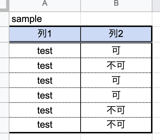
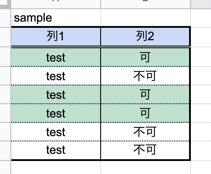
As in the Excel version of the article, set the background color, etc. for each row only for the row that is marked “Allowed” in “Column 2”, as shown in the figure below.
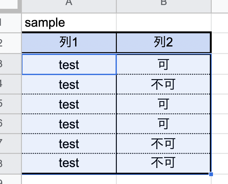
- Select the entire target range.
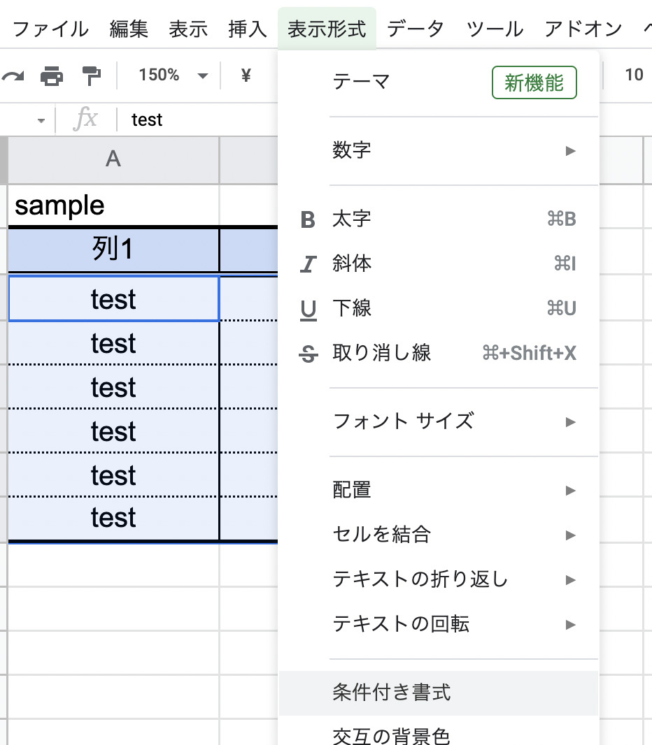
- With it selected, select “Conditional Formatting” in the “Display Format” tab.
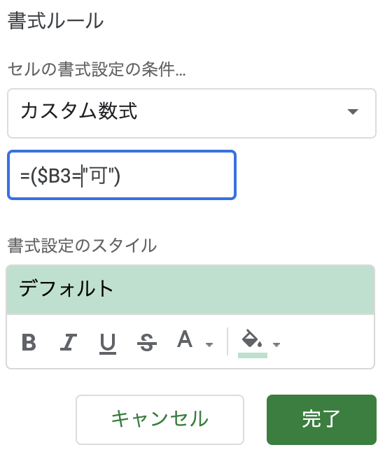
- When the condition setting screen appears, select “Custom Formulas” under “Format Rules”.
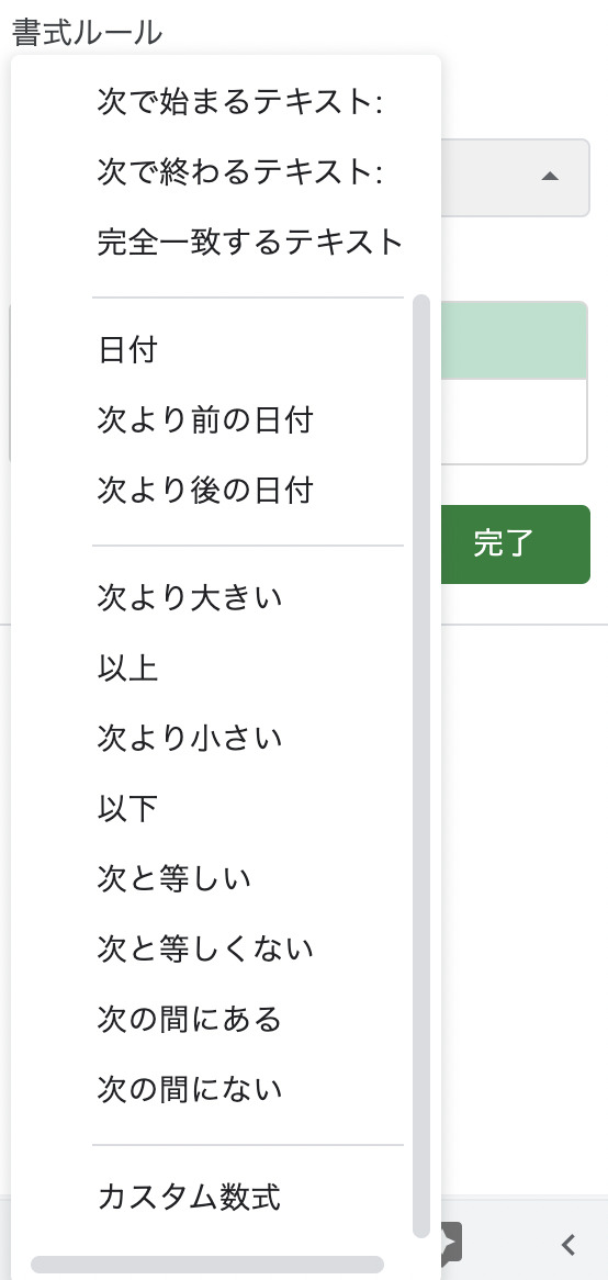
- In the same way as in the Excel version, enter “=$B3=”Yes” as a custom formula, set the format as desired, and click the “Finish” button.
In this case, the value “B3” is the location where you want the conditional branch to occur in the selected range.
- After completing the settings as described in the procedure, we can see that the conditional formatting has been set for the entire row with the word “allowed” in column 2.
How to operate in the Excel version
In this article, I showed you how to use the Google Spreadsheet version, but the following article will show you how to do the same operation in Excel. The way to use conditional formatting is quite different from the Google Spreadsheet version, so please check it out just in case.

conclusion
In this article, I introduced a procedure to apply conditional formatting in a spreadsheet to an entire row when the specified condition is met.
It is recommended to set the selection range not only to the created table but also to all columns, etc., so that the formatting will be automatically applied when the word “acceptable” is mentioned in the future.
 VOICEROID+ Tomoe Minoyasu EX Download Version
I am Japanese, and my computer is set up in Japanese. So there may be some differences in the names of the buttons and windows.
I try to keep the information on this site (tamocolony) up-to-date, but please be aware that the information on this site may not be the most up-to-date, or the information itself may be incorrect. We take no responsibility for the content of this site. If you have any questions about an article or need to make corrections, please contact us via the Contact Us page.